
How an LLM Finds a Lower-Loss Solution
A matrix-first look at logits, cross-entropy, gradients, AdamW, and where learning-rate schedulers actually enter the training loop.
In this article
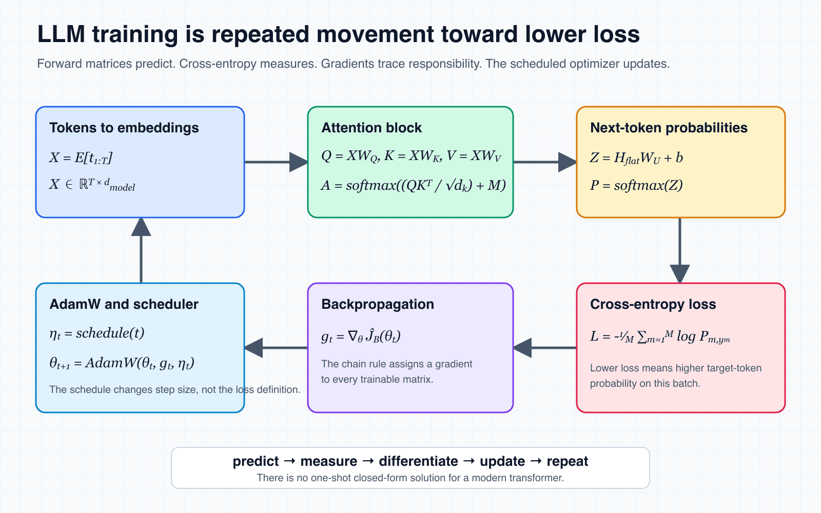
The short version
An LLM does not calculate one perfect global optimum in a clean closed-form equation. Training is too large, too noisy, and too non-convex for that. Instead, the model repeatedly moves toward lower loss on many batches of text. The practical target is a parameter region that predicts unseen text well, not proof that training found the deepest possible minimum.
The loop is simple in shape:
1. Run tokens through matrix operations.
2. Convert hidden states into next-token probabilities.
3. Measure error with cross-entropy loss.
4. Backpropagate gradients through the matrices.
5. Let an optimizer such as AdamW choose the parameter update.
6. Let a learning-rate scheduler scale the update over time.
Loss-landscape intuition
What optimum means in practice
In classical optimization, an optimum is the parameter setting that minimizes an objective function. For an LLM, the parameters are all learned weights. We can gather them into one huge vector:
θ = [WE, WQ, WK, WV, WO, W1, W2, WU, b, ...]
θ* = arg minθ J(θ)
Notation quick key
The objective Jis usually the expected next-token loss over the training data. We do not evaluate all possible text at once. We sample batches, calculate a noisy estimate of the loss, and update from that.
J(θ) = E(x,y)∼data [ L(fθ(x), y) ]
ĴB(θ) = (1 / B) Σi=1B L(fθ(xi), yi)
That is why people often say training is stochastic. Each batch is a small window into the whole data distribution. The optimizer is always steering from partial evidence.
A scheduler changes the path, not the destination formula
A gradient points downhill for the current batch. It does not say how far to travel. The learning rate supplies that distance, and the scheduler changes it over time.
The chart uses a simple two-parameter bowl so the path can be drawn. An LLM has billions of parameters and a much less regular surface, but the step-size problem remains. A learning rate that is too large can bounce across a narrow valley or diverge. A very small rate can make safe but painfully slow progress. Warmup and decay try to use different step sizes at different phases.
What the graph does and does not show
From tokens to matrices
Start with a tiny sequence of tokens. The tokenizer turns text into token IDs. The embedding table turns each token ID into a vector.
[t1, t2, t3, ..., tT]
E ∈ ℝV × d_model
X = E[token_ids]
X ∈ ℝT × d_model
Here, V is the vocabulary size, Tis the sequence length, and d_modelis the width of each token representation.
Embedding intuition
The core matrix step: attention
A transformer block uses learned matrices to create queries, keys, and values. This simplified single-head view leaves out multi-head splitting, layer normalization, residual paths, and feed forward layers so the core matrix operation stays visible.
X ∈ ℝT × d_model
WQ ∈ ℝd_model × d_k, WK ∈ ℝd_model × d_k, WV ∈ ℝd_model × d_v
Q = XWQ, K = XWK, V = XWV
Attention compares every query with every key. The result is a square score matrix. For a decoder-style language model, a causal mask is added before softmax so each position can only use earlier positions and itself.
S = (QKT) / √dk + Mcausal
S ∈ ℝT × T
A = softmax(S)
H = AV
H ∈ ℝT × d_v
The Transformer paper introduced this scaled dot-product attention form. The scaling bysqrt(d_k)keeps dot products from becoming too large, which helps the softmax stay in a useful gradient range.
From hidden state to loss
After several transformer blocks, the model has a hidden vector for each token position. To predict the next token, it maps each valid hidden vector into vocabulary-sized logits.
H ∈ ℝB × T × d_model
WU ∈ ℝd_model × V
Hflat ∈ ℝM × d_model
Z = HflatWU + b
P = softmax(Z)
With tiny numbers, that final projection might look like this:
H_flat = [[0.2, -0.1],
          [0.7,  0.3]]

W_U = [[1.0, -0.5,  0.2],
       [0.4,  0.8, -0.3]]

b = [0.1, 0.0, -0.2]

Z = H_flat W_U + b
Z = [[0.26, -0.18, -0.13],
     [0.92, -0.11, -0.15]]
A logit is an unnormalized score for a token. Softmax converts those scores into probabilities. Here, M is the number of valid next-token prediction positions after padding and ignored positions are removed.
Suppose the three vocabulary columns are [puppy, runs, .], and the two correct targets are [runs, puppy]. Softmax and cross-entropy give:
P = softmax(Z)
P = [[0.4308, 0.2775, 0.2917],
     [0.5882, 0.2100, 0.2018]]

L = -[log(0.2775) + log(0.5882)] / 2
L = 0.9063Lm = -log P[m, ym]
L = -(1 / M) Σm=1M log P[m, ym]
L = -(1 / M) Σm=1M Σv=1V Y[m,v] log P[m,v]
Lower loss means the model assigned higher probability to the true next tokens in the training batch. The whole training loop exists to change the matrices so this number tends to go down.
A concrete gradient calculation
The cleanest place to see the gradient is the final vocabulary projection. For the flattened valid prediction positions, letY be the one-hot matrix of correct tokens. A useful cross-entropy plus softmax result is:
P = softmax(Z)
Y ∈ ℝM × V
dL / dZ = (P - Y) / M
If the correct token should have probability 1 but the model gives it 0.30, that token gets a negative correction. If the model gives too much probability to a wrong token, that wrong token gets a positive correction. The gradient says how the logits should move.
For the two-row example above, the numerical logit gradient is:
G_Z = (P - Y) / 2
G_Z = [[ 0.2154, -0.3613,  0.1458],
       [-0.2059,  0.1050,  0.1009]]
Now apply the matrix derivative for the output matrix:
Z = HflatWU + b
GZ = dL / dZ
dL / dWU = HflatTGZ
dL / db = sum_rows(GZ)
dL / dHflat = GZWUT
This is the key mechanical idea. The model output was made by matrix multiplication, so the correction is also expressed through matrix multiplication. Backpropagation keeps applying the chain rule backward through every matrix, softmax, normalization, residual connection, and feed forward layer.
Applying that multiplication to the toy matrices produces:
dL/dW_U = H_flat^T G_Z

dL/dW_U = [[-0.1010,  0.0012, 0.0998],
           [-0.0833,  0.0676, 0.0157]]

dL/db = [0.0095, -0.2563, 0.2467]
Gradient intuition
The optimizer step
Once backpropagation has produced gradients for all parameters, collect them into one gradient object:
θt
gt = ∇θ ĴB(θt)
The simplest update is stochastic gradient descent:
θt+1 = θt - ηtgt
The learning rate η_tcontrols the step size. In large transformer training, Adam or AdamW is more common because it keeps moving averages of gradients and squared gradients.
mt = β1mt-1 + (1 - β1)gt
vt = β2vt-1 + (1 - β2)(gt ⊙ gt)
m̂t = mt / (1 - β1t)
v̂t = vt / (1 - β2t)
θt+1 = θt - ηt m̂t / (√v̂t + ε)
Adam changes the effective step per parameter. If one weight has repeatedly noisy or large gradients, its squared-gradient estimate can reduce the step. If another weight has a cleaner direction, it can move more confidently.
AdamW adds decoupled weight decay. Instead of mixing weight decay into the adaptive gradient calculation, it applies parameter shrinkage as a separate part of the update.
θt+1 = (1 - ηtλ)θt - ηtm̂t / (√v̂t + ε)
The practical effect is that the model still follows the gradient, while the optimizer also discourages weights from growing without bound. The AdamW paper is specifically about why this decoupling matters for adaptive optimizers such as Adam.
Training code often excludes bias and normalization parameters from weight decay. AdamW does not decide that policy by itself. Parameter groups in the training recipe decide which tensors receive which learning rate and decay value.
Where schedulers come into play
In image generation, a sampler scheduler often controls a denoising trajectory. In LLM training, the common scheduler is different: it controls the learning rate over training steps.
θt+1 = OptimizerStep(θt, gt, ηt)
ηt = schedule(t)
The scheduler does not usually decide the gradient direction. Backpropagation does that. The scheduler decides how strongly the optimizer should trust that direction at this stage of training.
| Schedule | Formula sketch | Training behavior |
|---|---|---|
| Constant | ηt = η0 | Simple, but can be too aggressive early or too high late. |
| Linear warmup | ηt = ηmax · t / w, for t ≤ w | Starts cautiously while gradients and optimizer moments stabilize. |
| Inverse square root | ηt ∝ 1 / √t | Used in the original Transformer schedule after warmup. |
| Linear decay to zero | ηt = ηpeak(1 - p) | Reduces the rate evenly after warmup and reaches zero at the planned end. |
| Cosine decay | ηt ∝ 1 + cos(πp) | Stays higher early and bends gently toward a small final rate. |
| Warmup-stable-decay | warmup, plateau, cooldown | Keeps a reusable high-rate training branch, then decays near a chosen endpoint. |
After a warmup of wsteps in a run planned to end atT, define post-warmup progress as:
p(t) = (t - w) / (T - w), for w ≤ t ≤ T
ηlinear(t) = ηpeak(1 - p(t))
ηcosine(t) = ηmin + ½(ηpeak - ηmin)(1 + cos(πp(t)))
ηinverse-sqrt(t) = ηpeak√(w / t)
Warmup-stable-decay keepsη = η_peakthrough a stable middle phase, then applies a chosen cooldown curve over the final segment. The name describes the phases, not one mandatory cooldown equation.
The original Transformer paper used Adam with a warmup plus inverse-square-root schedule:
ηt = dmodel-0.5 · min(t-0.5, t · warmup_steps-1.5)
Before warmup ends, the second term grows linearly with step. After warmup, the first term decays as training progresses. This gives the optimizer a gentle start and then smaller refinement steps.
There is no universally best curve. The original Transformer used inverse-square-root decay. Cosine decay became common in later training recipes. MiniCPM introduced warmup-stable-decay for a training horizon that can be extended before cooldown. A 2025 empirical study reported that, under its tested compute-optimal settings and tuned peak rates, linear decay to zero outperformed the compared tenfold-decay schedules. That result is evidence for a recipe, not a proof for every dataset, model size, optimizer, or fine-tuning run.
Training-speed intuition
A tiny numerical example
We can now close the loop on the toy output matrix. Hold the hidden states fixed and apply one plain SGD update with learning rate 0.1 toW_U andb.
W_U' = W_U - 0.1(dL/dW_U)
b'   = b   - 0.1(dL/db)

W_U' = [[ 1.0101, -0.5001,  0.1900],
        [ 0.4083,  0.7932, -0.3016]]

b' = [0.0990, 0.0256, -0.2247]
Recompute the logits and probabilities with those updated values:
P' = [[0.4310, 0.2849, 0.2841],
      [0.5911, 0.2142, 0.1947]]

L_before = 0.9063
L_after  = 0.8907
The loss fell for this batch because the step followed its gradient and was small enough. This is a local demonstration, not a guarantee that every batch or validation example improves after every update. In a full model, backpropagation updates all trainable matrices, AdamW rescales the coordinate-wise update, and the scheduler changes the learning rate across training.
Why there is no simple closed-form answer
If this were ordinary linear regression, we could sometimes solve for the best weights with a compact matrix equation. LLMs are different:
- The model contains many nonlinear operations, including softmax, activation functions, and normalization.
- The training objective is non-convex, so there are many basins, saddles, and flat regions.
- The data is sampled in batches, so each gradient is noisy.
- The model is overparameterized, so many different parameter settings can behave similarly.
- The goal is useful generalization, not only perfect memorization of the training set.
So the useful mental model is not one grand equation that produces the final LLM. It is an iterative machine: matrix prediction, loss measurement, gradient calculation, optimizer update, scheduled step size, repeat.
Training loss is also not the whole product objective. Teams monitor validation loss, downstream evaluations, safety behavior, calibration, and overfitting. A lower training loss can be mathematically real while the model becomes less useful on data it did not train on.
Sources
This article is a simplified explanation, but the core formulas are grounded in the standard transformer and optimizer literature.
- Attention Is All You Need for scaled dot-product attention, transformer architecture, Adam use, and the original warmup plus inverse-square-root learning-rate schedule.
- Adam: A Method for Stochastic Optimization for first and second moment estimates, bias correction, and the Adam update rule.
- Decoupled Weight Decay Regularization for AdamW and the distinction between L2 regularization and decoupled weight decay.
- SGDR: Stochastic Gradient Descent with Warm Restarts for the cosine annealing schedule.
- MiniCPM: Scalable Training Strategies for warmup-stable-decay in language-model training.
- Straight to Zero for the empirical comparison of linear decay to zero with common LLM schedules.
- PyTorch AdamW documentation for a current implementation reference and the decoupled weight-decay update.
Keep reading
Related articles

What MiniMax H3 Is Actually Good At
See when MiniMax H3 preserves finished designs better than WAN 2.2 and LTX 2.3, when that restraint becomes a weakness, and how its audio and references behave.
Why AI Video Is So Much Heavier Than AI Images
Understand why AI video needs more GPU memory and compute than image generation, with tensor math, frame-resolution scaling, temporal attention, and practical cost controls.